Faster String Search: The Recall Trade-off Behind a 20x Speedup

Revised 7 September 2026. The original benchmark table and charts are unchanged. This revision clarifies the approximate-search contract and corrects the cost comparisons. No new benchmark run is reported here.

I built a string similarity search algorithm a while back. The idea was simple: compute a reusable fingerprint for each string, use those fingerprints to select candidates, then run expensive edit-distance comparisons on the shortlist.

It ran roughly 13–20x faster than my exhaustive baseline across the workloads below. It also missed some of the true nearest neighbours. For the 100,000-string workload with 100-character strings, the reported result is 17.5x faster at 89% recall.

Later, I noticed a connection with retrieval-augmented generation. Both put a cheaper selection stage ahead of expensive downstream processing. That connection led me to other systems with a similar instinct: spend a little now to avoid spending much more later.

The differences between those systems matter. Some filters can safely exclude a candidate. My proxy can exclude the correct answer. Speculative execution has a recovery mechanism for a wrong guess. Those contracts determine how far the analogy travels.

The Problem

Take a corpus of 100,000 strings. Given a query, the exact task is to find the ten closest strings by Levenshtein edit distance.

My filtered search returns the closest matches within its selected candidate set. A string rejected by the proxy receives no exact comparison. Scoring the survivors exactly leaves that earlier selection error intact.

For equal-length strings, the standard dynamic-programming recurrence evaluates O(L²) cells per comparison. At 100 characters per string, an exhaustive scan involves roughly:

100,000 x 100 x 100 = 1,000,000,000 DP-cell updates

The original measurement for that workload was about 1.4 seconds per query. That made a cheap screening stage worth investigating.

This is a comparison against my exhaustive implementation. Other exact methods include bit-parallel algorithms and banded methods when a useful distance bound is available. The table does not establish a speedup against every optimised exact-search implementation.

The Extra Stage

The benchmark description uses a fixed-size fingerprint of about 182 floats per string. It combines character statistics with positional information. Those features are computed before the query workload and reused.

At query time:

1. Encode the query using the same features.
2. Scan the stored feature vectors and compute squared L2 distances.
3. Keep the closest 5% by that proxy distance.
4. Evaluate Levenshtein on the retained strings and select the requested results.

For the 100K workload, that means screening 100,000 feature vectors before making about 5,000 edit-distance comparisons. The extra stage removes most of the calls to the expensive kernel.

The earlier version added float-coordinate counts to DP-cell counts and treated the sum as a performance prediction. That comparison mixed different units of work. A subtract-square-accumulate operation and a DP-cell update have different costs. Instruction dependencies matter, as does memory traffic.

The hardware explanation needs the same discipline. A linear feature scan has predictable accesses and simple arithmetic that are suitable for vectorisation. That does not establish achieved instructions per cycle or eliminate cache misses. My benchmark timings alone cannot tell us how far ahead the prefetcher ran.

Levenshtein's recurrence carries dependencies between neighbouring cells. The amount of dependent work per candidate is the relevant contrast here. We do not need to assume a materialised two-dimensional table to explain the recurrence.

The practical gain comes from avoiding most expensive comparisons while keeping selection cheap. Profiling the individual stages would tell us how much of the remaining time is spent scanning features and how much is spent elsewhere.

The Numbers

These are the original reported measurements: single-threaded, compiled with -O3 -march=native, on Apple Silicon. They are retained here without a fresh run.

scenario             |  brute lev  | filter+lev  | feat only  | speedup | recall
---------------------+-------------+-------------+------------+---------+--------
1K  x  20-char       |      369 us |       26 us |      15 us |   14.0x |  86.5%
1K  x 100-char       |   12,496 us |      653 us |      19 us |   19.1x |  97.5%
1K  x 500-char       |  317,581 us |   16,101 us |      23 us |   19.7x | 100.0%
10K x  20-char       |    3,639 us |      267 us |     159 us |   13.6x |  88.5%
10K x 100-char       |  117,595 us |    6,072 us |     204 us |   19.4x |  91.5%
10K x 500-char       | 3,246,553 us |  159,475 us |     212 us |   20.4x |  98.0%
100K x  20-char      |   39,865 us |    3,012 us |   2,888 us |   13.2x |  87.0%
100K x 100-char      | 1,394,453 us |   79,610 us |   4,303 us |   17.5x |  89.0%

The 100K-by-100-character row combines a 17.5x speedup with 89% reported recall. That percentage should not be read as the fraction of queries returning a completely correct top ten. The precise recall calculation and treatment of equal-distance ties still need to be documented from the benchmark implementation.

The feature configuration also needs to be pinned alongside the benchmark revision. The 182-float description here records the original benchmark account; it should not be used as a statement about the current library's default encoder or supported character set.

Longer strings make the edit-distance comparisons more expensive while the feature dimension stays fixed. That explains why filtering has more room to pay for itself as string length increases. It does not establish that every longer-string dataset will have better recall.

The "feat only" column shows that screening was a small part of the measured elapsed time on most of these workloads. It does not include a complete attribution of allocation or candidate-selection overhead.

The filter percentage controls how many candidates survive. Increasing it gives previously rejected candidates a chance to enter the final result. The speed cost and recall benefit need to be measured together. Their shape depends on the workload.

The original charts below report 100 queries per configuration on a 10K corpus. The runs used a deterministic seed and the same compiler flags.

Recall and Speedup vs String Length

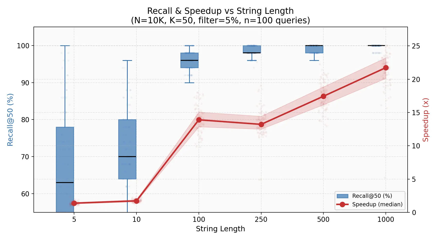
Recall and speedup improved with string length in this sweep. Recall exceeded 96% for strings of at least 100 characters, and speedup exceeded 14x. The fixed-size fingerprint had less useful ranking information on the shortest strings.

Recall and Speedup vs K

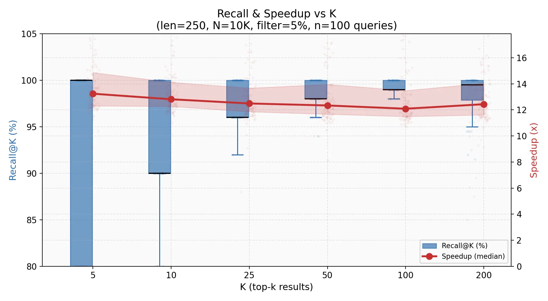
Reported recall stayed above 92% over the tested K values, from 5 through 200. Speedup stayed around 13x while the candidate pool remained fixed at 500 strings. Changing the requested result count did not change how many candidates received an edit-distance comparison in this sweep.

Recall and Speedup vs Filter Percentage

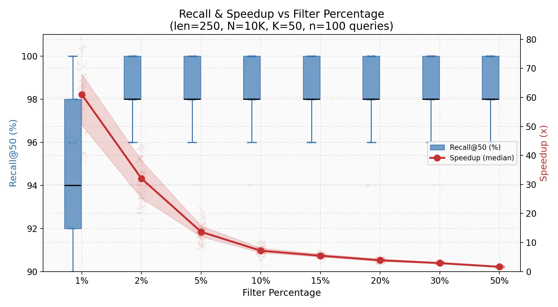
The filter-percentage sweep reported 94% recall with a 65x speedup at 1% filtering, compared with 98.5% recall and a 15x speedup at 5%. Moving from 1% to 10% candidates raised reported recall from 94% to 99%.

Those are observations from that sweep. They do not support a general promise that recall is cheap to recover. An application needing the missing neighbours may reject the faster configuration outright.

The Formal Principle

Let $N$ be the corpus size and $\varepsilon$ the survivor fraction in a simplified model. Use consistently measured costs: $c_f$ for filtering one item and $c_e$ for an expensive comparison.

$$T_{\mathrm{brute}} = Nc_e$$ $$T_{\mathrm{filtered}} = Nc_f + \varepsilon Nc_e$$

The model assumes uniform per-item costs and leaves out fixed query overhead. It gives the speedup:

$$S = \frac{1}{c_f/c_e+\varepsilon}$$

Filtering wins under those assumptions when:

$$\frac{c_f}{c_e} < 1-\varepsilon$$

The earlier substitution of 182 feature coordinates and 10,000 DP cells did not estimate $c_f/c_e$. Both costs need a common unit, such as elapsed time measured under comparable conditions.

A fuller accounting includes query encoding and candidate selection. The exact comparisons then run on the candidate set $C(q)$, followed by final result selection:

$$T(q)=T_{\mathrm{encode}}(q)+T_{\mathrm{scan}}(N,d)+T_{\mathrm{select}}(N,m)+\sum_{i\in C(q)}T_{\mathrm{edit}}(q,s_i)+T_{\mathrm{topk}}(m,k)$$

Here $m$ is the candidate count and $k$ is the requested result count. This decomposition identifies costs to measure; it does not assign timings we have not collected.

Preprocessing also belongs in the economics. If a built representation is reused for $Q$ queries, the amortised cost per query is:

$$\frac{T_{\mathrm{build}}}{Q}+T(q)$$

A one-query workload can therefore have a different winner from a heavily reused index.

The simple model also puts a ceiling on the predicted speedup. With a 5% survivor fraction and positive filtering cost, it predicts less than 20x. The table's 20.4x row shows the limits of applying uniform per-candidate costs to measured executions. It does not justify assigning the difference to an unmeasured hardware effect.

Recall sits outside this latency equation. A fast configuration that misses required matches fails the application. The useful decision is which configuration meets the quality requirement at an acceptable cost.

The Connection to RAG

Retrieval-augmented generation selects material before the language model processes it. That is the structural connection that caught my attention.

The document representation serves a role similar to my string fingerprint: it makes a preliminary selection affordable. After that point, the pipelines diverge. My expensive stage computes a distance for each retained string. A RAG generator consumes the retrieved context to produce an answer.

The generator has no automatic guarantee of factual correctness. Calling it "the expensive verifier" gave the architecture a property it does not possess.

Its costs differ too. Retrieval and any reranking precede context processing and generation. Context length affects that downstream work, and output length introduces another cost. Applying a constant per-document edit-distance model to the generator hides those differences.

The shared idea remains useful: select information before spending heavily on it. The correctness of the eventual answer still needs its own evidence.

When the Cheap Stage Is Wrong

A conventional Bloom filter can reject an absent key without rejecting an inserted key, assuming the structure is used correctly. A false positive sends unnecessary work downstream. My approximate shortlist has a different failure: a false negative removes a genuine neighbour before exact scoring begins.

These are different reasons to trust a rejection. A conservative bound establishes that a candidate cannot matter. A heuristic score only suggests that spending time on it is unlikely to help.

That distinction also matters for cascades. Viola and Jones use cheap early stages to reject many image windows before later classification work. Detection quality is part of the contract. Multiplying conditional false-positive rates across stages describes one side of the trade-off; detection rates compound too.

My original sequence of stage feature counts should not have been presented as the published detector. Likewise, $0.5^{30}$ is an illustrative product that requires a conditional false-positive rate of one half at every stage. It is not a general description of a trained cascade.

Speculation Saves Serial Time

Speculative decoding proposes a block of future tokens and evaluates the proposed trajectory with the target model. Its acceptance-and-correction procedure preserves the target model's output distribution under the algorithm's assumptions.

That guarantee concerns sampling from the target distribution. It does not certify the factual correctness of generated text.

The opportunity is to reduce serial target-model steps through parallel verification. A draft model's cost and acceptance rate alone do not determine the speedup. Draft length matters, along with the cost of verifying the block. My earlier substitution into the filter-refine equation left out those dependencies, so the numerical prediction has been removed.

CPU speculation has a related critical-path motivation. A branch prediction lets execution proceed before the branch resolves. A wrong prediction can require discarding work and recovering. A correct prediction still uses hardware resources; calling it zero-overhead was unjustified.

Filtering avoids selected computations. Speculation changes when work can proceed and how errors are corrected. A similar preliminary decision can serve a different performance mechanism.

Ordering Work in a Database

Many database plans use indexes or summaries to avoid unnecessary work. A plan can also choose a scan. The choice depends on the query and its estimated costs, so "every query plan does this" was too broad.

Hellerstein and Stonebraker's predicate migration work considers the placement of expensive predicates. Cost and selectivity both matter. A more expensive predicate can deserve an earlier position when it rejects enough work to reduce the total cost.

That is the useful lesson for the analogy: judging a stage by its own cost alone misses the work it prevents later.

Sequential testing addresses a related decision about whether to gather more evidence or stop. Its optimality results belong to specified statistical problems. My original claim that Wald proved a universally optimal version of cheap-before-expensive computation was too broad.

What the Representation Buys

The fingerprint is larger than the source in the 100-byte example: 182 float32 values occupy 728 bytes. Its purpose is to make a later selection decision cheaper. Calling it lower-dimensional or smaller without specifying the representation confused that purpose with storage compression.

The encoder must inspect the input to build its features. Reuse is where the benefit appears: later queries compare the prepared representation rather than repeating the expensive computation for every string.

A useful proxy retains enough ranking information for the shortlist. Average correlation with edit distance is insufficient if the closest matches are repeatedly lost. Positional summaries also discard distinctions in character order. That is a reason to examine failure cases rather than treating high recall on a particular dataset as a property guaranteed by the representation.

Document embeddings face the same practical question about which distinctions retrieval preserves. My earlier claim that their losses are orthogonal to relevance had no supporting guarantee. Retrieved evidence must be checked against the actual query.

Speculative decoding has a separate protection: the correction rule preserves the target distribution. It does not need an assumption that rare outcomes are noise.

The recurring opportunity is a cheap preliminary decision that changes the cost of subsequent work. Its value depends on the errors it makes and what the rest of the system does with those errors.

What I Would Take From This

The string experiment demonstrates a useful approximate-search trade-off on the reported workloads. Its strongest result is the measured combination of latency and recall.

The cross-domain connection becomes more useful once its boundaries are explicit. For a new system, identify the work the extra stage saves. Then examine how a wrong preliminary decision affects the result.

Keep those questions attached to the measurements. Otherwise it is easy to recognise a familiar shape and carry the wrong guarantee across with it.

Including me.

The string similarity library is open source: github.com/NagyErvin-ZY/fast-comapre-simdstring