When More Is Faster: How Doing Extra Work Gives You a 20x Speedup

I built a string similarity search algorithm a while back. The core idea was dead simple: instead of comparing every string against every other string with expensive edit distance, pre-compute a cheap numerical fingerprint for each string, scan those fingerprints first, then only run the expensive comparison on the survivors.

It worked. 20x faster than brute force.

Years later, RAG showed up. Retrieval-Augmented Generation. The architecture: encode your documents into cheap vector embeddings, do a fast similarity search to find the relevant ones, then feed only those to the expensive LLM.

Same pattern. Exactly the same pattern.

Turns out I didn't invent anything. This pattern is one of the most fundamental ideas in computer science, and it has been independently discovered in almost every subfield. This post is about what that pattern is, why it works, when it breaks, and why it keeps showing up everywhere from CPU architecture to agentic AI systems.

The Problem

You have 100,000 strings. A user gives you a query string. Find the 10 closest matches by Levenshtein edit distance.

The standard Levenshtein DP is O(L²) time for equal-length strings. Faster exact variants exist in some regimes (bit-parallel, banded methods for bounded distances), but worst-case quadratic time is common. For 100K strings of 100 characters each, that's:

100,000 x 100 x 100 = 1,000,000,000 operations

On my machine, that takes 1.4 seconds per query. For an interactive system, that's dead.

The Counterintuitive Solution: Do More Work

Here's the trick that shouldn't work but does. For every string in the corpus, pre-compute a fixed-size feature vector. This vector captures the statistical fingerprint of the string: character frequencies, positional distributions, binned presence patterns. About 182 floats per string.

At query time:

1. Encode the query into the same 182-float vector
2. Scan ALL 100K feature vectors and compute L2 distance (cheap: just subtract-and-square 182 floats per string)
3. Take the top 5% by feature distance (5,000 strings)
4. Run actual Levenshtein ONLY on those 5,000 survivors

The total operation count is higher than brute force. You're doing the feature scan (100K x 182 = 18.2M ops) ON TOP of the Levenshtein on survivors (5K x 10K = 50M ops). That's 68M operations versus the brute-force 1B.

Wait. That's fewer. The "more work" (the feature scan) replaced 95% of the expensive work. You did more things, but less total compute.

But there's a deeper reason it's fast, beyond the operation count.

The feature scan is 100,000 × 182 subtract-and-square operations on contiguous float arrays. That's data-oriented design in its purest form: data laid out exactly how the CPU wants to consume it. The feature store uses column-major storage — each feature dimension is a single contiguous array in memory. The CPU prefetcher sees a linear sweep and stays three cache lines ahead. SIMD instructions (NEON on Apple Silicon, AVX2 on x86) process 4-8 floats per clock cycle. No branches, no pointer chasing, no cache misses.

Levenshtein is the opposite. A 2D dynamic programming table where each cell depends on three neighbors. Loop-carried dependencies limit SIMD and instruction-level parallelism. The DP rows themselves have decent locality for moderate L, but brute-force iteration over 100K variable-length string allocations adds pointer chasing the feature matrix avoids entirely. The net result: much more work per candidate, and far less of the hardware's throughput utilized.

On its face, "do extra work to go faster" sounds like nonsense. This is why face-value reasoning fails in systems programming. "More operations" doesn't mean slower. A billion cache-friendly SIMD float subtractions completes faster than a hundred million dependency-heavy DP cells. Big-O notation tells you scaling behavior. It tells you nothing about the constant factor — and that constant varies by 100x depending on whether your memory access pattern aligns with the hardware sitting on the die.

The Numbers

These are real measurements, not estimates. Single-threaded, -O3 -march=native, Apple Silicon:

scenario             |  brute lev  | filter+lev  | feat only  | speedup | recall
---------------------+-------------+-------------+------------+---------+--------
1K  x  20-char       |      369 us |       26 us |      15 us |   14.0x |  86.5%
1K  x 100-char       |   12,496 us |      653 us |      19 us |   19.1x |  97.5%
1K  x 500-char       |  317,581 us |   16,101 us |      23 us |   19.7x | 100.0%
10K x  20-char       |    3,639 us |      267 us |     159 us |   13.6x |  88.5%
10K x 100-char       |  117,595 us |    6,072 us |     204 us |   19.4x |  91.5%
10K x 500-char       | 3,246,553 us |  159,475 us |     212 us |   20.4x |  98.0%
100K x  20-char      |   39,865 us |    3,012 us |   2,888 us |   13.2x |  87.0%
100K x 100-char      | 1,394,453 us |   79,610 us |   4,303 us |   17.5x |  89.0%

Two things to notice:

The speedup increases with string length. Levenshtein is O(L²). The feature scan is O($d$) per string where $d$ is the fixed feature dimension — independent of original string length. The feature encoding already projected the string into a fixed-size vector. So the longer the strings, the more the expensive computation dominates, and the more the filter saves.

The "feat only" column is the real story. 100K strings in 4 milliseconds. The feature scan itself is absurdly fast because it's a SIMD-friendly linear sweep over contiguous float arrays. The Levenshtein rerank on the 5% survivors is where 95% of the pipeline's time goes.

Recall is a dial, not a fixed number. The 5% filter cutoff is a choice. Widen it to 10% and recall climbs — but the speedup drops sub-linearly, not linearly, because the feature scan cost is fixed and the Levenshtein cost on survivors grows smoothly. In general, the more data you throw at the expensive stage, the higher recall goes. The tradeoff curve is favorable: you give up speedup slowly and gain recall quickly. An interesting direction for further study would be investigating what specific features of the input data drive recall at a given top-k cutoff — which string properties cause the feature proxy to disagree with Levenshtein, and whether targeted feature engineering could close that gap.

The following charts show these dynamics across 100 queries per configuration on a 10K corpus (deterministic seed, -O3 -march=native, Apple Silicon):

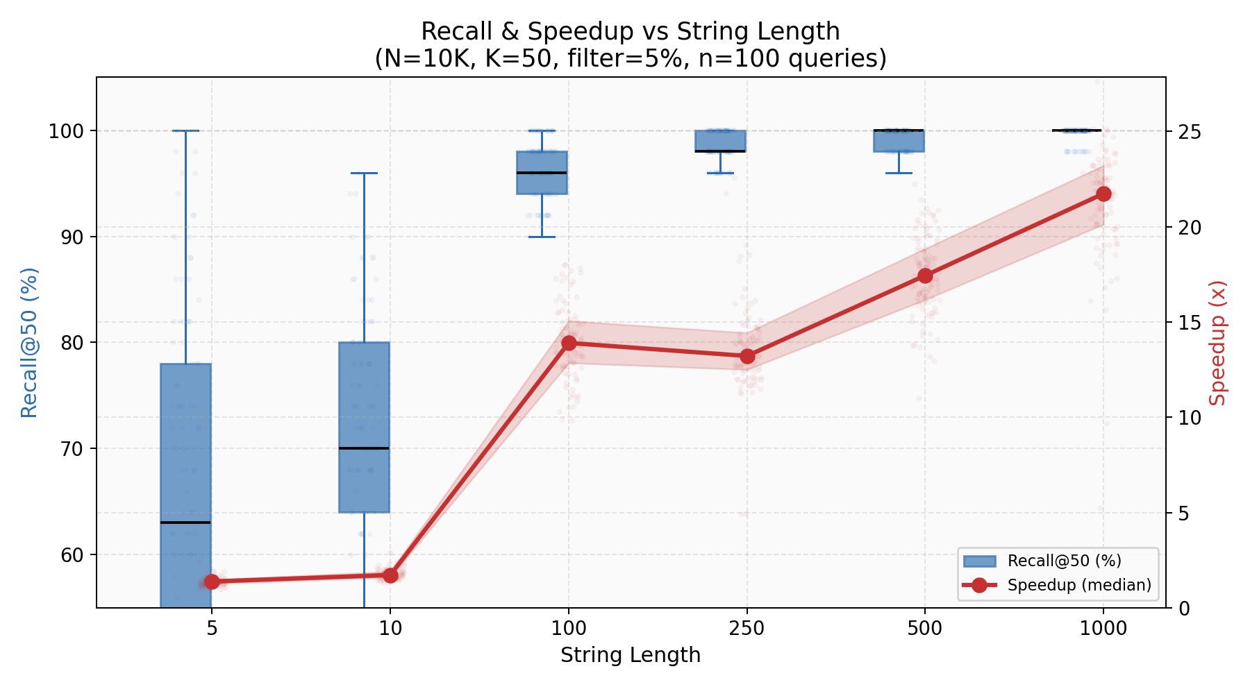
Both recall and speedup climb with string length. At length 5, the feature vector has almost nothing to work with — 5 characters projected into 182 floats is noise. By length 100+, recall exceeds 96% and speedup passes 14x. The O(L²) Levenshtein cost dominates harder as strings grow, making the fixed-cost feature scan proportionally cheaper.

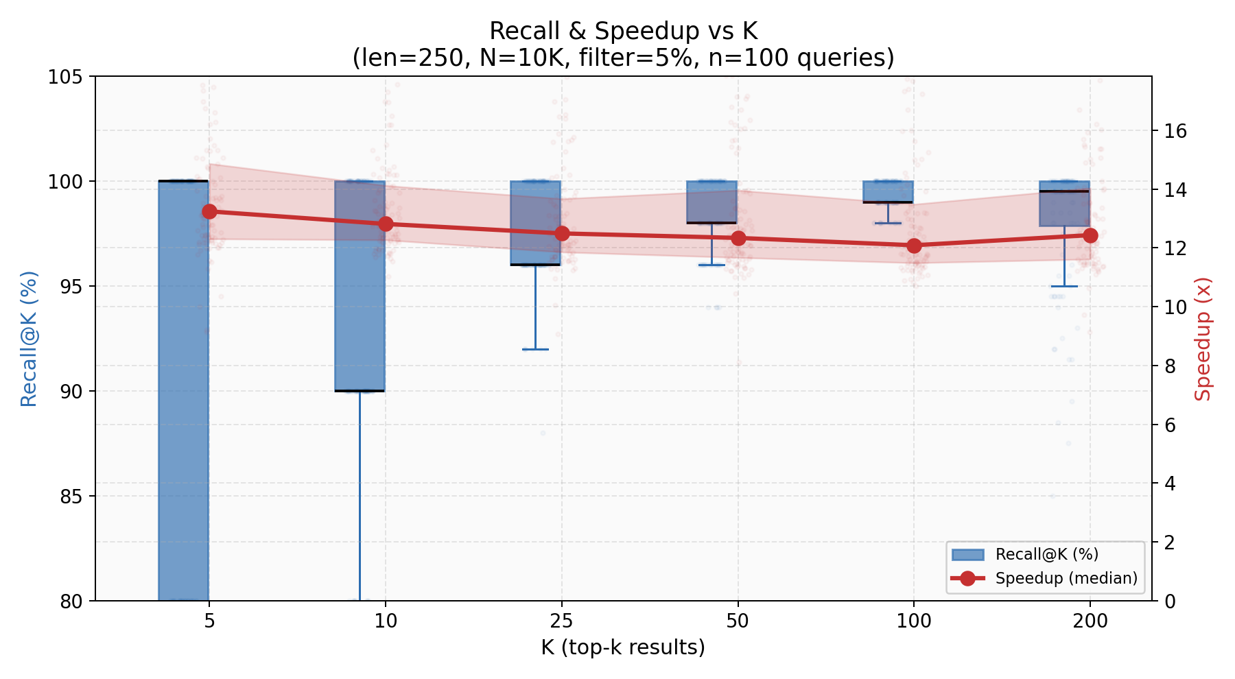
Recall stays above 92% across all tested K values (5 through 200), with the median tightening as K grows — the algorithm has more room to be approximately right. Speedup is stable around 13x regardless of K, because the bottleneck is always the Levenshtein rerank on the fixed 500 candidates (5% of 10K).

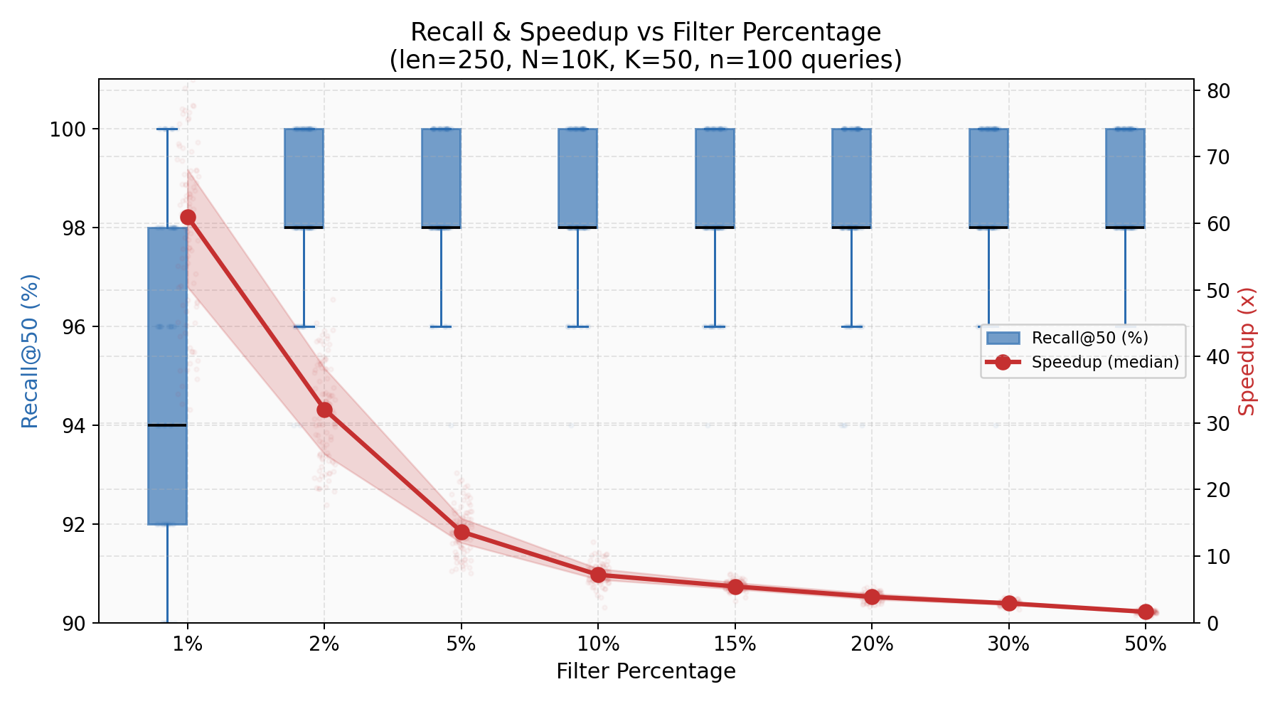
The tradeoff knob. At 1% filter (100 candidates), recall is already 94% with a 65x speedup. At 5% (500 candidates), recall hits 98.5% with 15x speedup. The curve is asymmetric: recall saturates quickly while speedup degrades smoothly. You can dial recall from 94% to 99% by going from 1% to 10% filter — a 10x increase in candidates for 5 percentage points of recall.

Wait. This Is RAG.

Here's what RAG does:

1. Pre-compute dense vector embeddings for all documents in the corpus
2. At query time, encode the query into the same embedding space
3. Fast vector similarity search to find the top-k most relevant documents
4. Feed ONLY those documents to the expensive LLM for synthesis

Replace "documents" with "strings," "embeddings" with "feature vectors," "vector similarity" with "L2 distance on feature vectors," and "LLM" with "Levenshtein distance."

It's the same architecture.

The RAG paper (Lewis et al., 2020) formalized this for language models. But the pattern predates it by decades. The string similarity library I built uses the same filter-refine architecture that PostgreSQL's pg_trgm extension has shipped since 2005, which itself uses the same candidate-generation-and-verification pattern from Karp-Rabin string matching (1987).

In the current wave of agentic AI systems, RAG is the backbone of how agents access knowledge. An agent doesn't feed its entire knowledge base to the LLM on every step. It retrieves a small relevant subset first — cheap computation on everything, expensive computation on the survivors. The agent's retrieval system IS a filter-refine pipeline. The vector database IS the feature store. The LLM IS the expensive verifier.

The parallel isn't a metaphor. It's structural.

Wait. This Is Everything.

Once you see the pattern, you can't unsee it.

Speculative decoding in LLMs (Leviathan et al., 2023). A small, fast "draft" model generates K candidate tokens. The large target model verifies all K tokens in a single batched forward pass. Cheap bulk generation, expensive verification on the output. If the draft model's acceptance rate is high, you get 2-3x inference speedup with mathematically identical output distribution. The draft model is the filter. The target model is the verifier.

CPU speculative execution. The branch predictor guesses which way a conditional will go (cheap: a lookup in a history table). The CPU executes instructions along the predicted path speculatively. If right (95-99% of the time), zero overhead. If wrong, flush the pipeline and re-execute (expensive, but rare). Same pattern. Cheap prediction on all branches, expensive correction on the mispredictions.

Viola-Jones face detection (2001). A cascade of increasingly expensive classifiers. Stage 1: two simple Haar features reject 50% of candidate windows. Stage 2: five features on the survivors. Stage 3: twenty features. By stage 30, the false positive rate is 0.5³⁰ — essentially zero. The average number of features evaluated per window is about 10, even though the full classifier has thousands of features. The first stages are the cheap filter. The later stages are the expensive verifier.

Database query optimization. Every query plan does this. The B-tree index scan (cheap) identifies candidate rows. The full predicate evaluation (expensive) runs only on candidates. Bloom filter joins reject non-matching rows before the expensive probe. Zone maps eliminate entire disk blocks with a single min/max comparison. The 1993 paper by Hellerstein and Stonebraker ("Predicate Migration") literally formalizes the optimal ordering of cheap-before-expensive predicates.

Bloom filters (1970). A probabilistic data structure that says "definitely not in the set" or "maybe in the set." The cheap Bloom filter lookup avoids the expensive disk I/O or network call for guaranteed negatives. Every LSM-tree database (LevelDB, RocksDB, Cassandra) uses this on every read.

Every single one of these is the same architecture: cheap computation on everything, expensive computation on the survivors.

The Formal Principle

The core inequality is simple: filter-refine wins when the filter's cost ratio to the expensive computation is less than its rejection rate.

where $c_f$ is the per-item filter cost, $c_e$ is the per-item expensive cost, and $\varepsilon$ is the fraction of candidates that survive. For my string search, $c_f = 182$ float ops, $c_e = 10{,}000$ ops (100-char Levenshtein), $\varepsilon = 0.05$:

The condition is satisfied by a factor of 50 — the filter could be 50x more expensive and still worth it.

This also explains when the pattern breaks: when strings are short ($c_e$ isn't large enough to justify the overhead) or when selectivity is low (the filter can't reject enough candidates, so $\varepsilon$ approaches 1).

The formal mathematics behind optimal filter ordering goes deep. Abraham Wald's Sequential Probability Ratio Test (1945) proves the optimal strategy for staged evidence gathering. Hellerstein and Stonebraker's "Predicate Migration" (1993) formalizes optimal cheap-before-expensive predicate ordering in databases. The Viola-Jones cascade (2001) extends it to multi-stage classifiers. The concept appears under different names in every subfield — filter-refine, coarse-to-fine, cascade, prune-and-search, branch-and-bound — but the underlying inequality is always the same.

Why It Keeps Working: Information Is Compressible

The deeper question is: why do cheap proxies have high recall in the first place? Why does a 182-float feature vector preserve the ranking of a 10,000-operation edit distance computation?

Because real-world data has structure, and structure is compressible.

A 100-byte ASCII string is 800 bits of raw information. The feature vector (182 float32s = 728 bytes) isn't smaller in raw size — it's a fixed-size projection that retains the task-relevant signal. Edit-distance-relevant information — which characters a string contains, where they appear, how they're distributed — lives in a much lower-dimensional subspace than the full string. The feature vector is a lossy projection from the string space into a $d$-dimensional float space (here $d = 182$). The loss is concentrated in dimensions orthogonal to "similarity" — the exact order of characters within a positional bin, for example.

This is the same reason RAG works. A document has thousands of tokens, but its "relevance to a query" can be approximated by a 768-dimensional embedding. The embedding is a lossy compression of the document, but the loss is concentrated in dimensions orthogonal to relevance.

And it's the same reason speculative decoding works. The draft model is a "compressed" version of the target model. It captures the high-probability token predictions (the structured part) and misses the low-probability edge cases (the noisy part).

The pattern works whenever:

1. The expensive computation depends on a compressible signal in the input
2. A cheap proxy can extract that signal without processing the full input
3. The proxy has high recall — it preserves the top of the ranking, even if the exact distances are wrong

When these conditions hold, you get the seemingly paradoxical result: doing more total work produces a faster system, because the extra work is cheap and it eliminates most of the expensive work.

The Generalized Model

Here's the recipe, abstracted from all the instances. Given $N$ items, per-item expensive cost $c_e$, per-item filter cost $c_f \ll c_e$, survivor fraction $\varepsilon$, and filter recall $\rho$:

For my string search:

Measured: 13-20x depending on scenario.

For RAG: retrieval is typically milliseconds per query (an ANN index lookup plus optional rerank), while generation is tens to thousands of milliseconds depending on model and output length. The qualitative inequality $c_f \ll c_e$ holds by orders of magnitude — and context-window limits make "feed the whole corpus" infeasible regardless of compute.

For speculative decoding: $c_f$ = draft model forward pass, $c_e$ = target model forward pass. The ratio is typically 10-50x. With an 80% acceptance rate, the theoretical speedup is ~3x. Measured: 2-3x. The math checks out.

The pattern is not a clever hack. It's a consequence of the fundamental property that most real-world computations depend on compressible signals, and cheap projections can extract those signals. It shows up everywhere because that property is everywhere.

I built a string search library and found a 20x speedup. Then RAG showed up and did the same thing with documents and LLMs. Then I looked around and realized CPUs, databases, compilers, graphics engines, face detectors, and LLM inference systems all do it too. The principle has been independently discovered so many times that it doesn't have a single canonical name — it's called filter-refine, coarse-to-fine, cascade, prune-and-search, speculative execution, or branch-and-bound depending on which building you're standing in. Wald proved the optimal version in 1945.

The one-sentence version: if you can build a cheap function that mostly agrees with your expensive function, run the cheap one on everything and the expensive one on the survivors. The math always works out. The speedup is always real. And somehow, every generation of engineers rediscovers it from scratch.

Including me.

The string similarity library is open source: github.com/NagyErvin-ZY/fast-comapre-simdstring